Across all of my professional positions, I have used Microsoft Excel extensively. Over the years I have learned some tips and tricks and have become an “accidental expert”. While working at Overdrive, Excel was the primary software that I utilized to normalize data submitted from publishers for upload to the database. At the library, I teach a beginner and intermediate level Excel class. It is one of the most popular computer classes that the library offers. I’ll demonstrate some of my Excel skills below.
Using Conditional Formatting in Excel
What is conditional formatting and why would you want to use it?
The conditional formatting tool is available on the Home tab in Excel.
![]()
Conditional formatting will highlight cells if they meet certain criteria – this can include identifying duplicate data, locating specific text, and discovering numbers that are above or below a certain range. It is useful in spotting trends. Once the cells are highlighted, it is then possible to sort or filter the data in the worksheet based on the newly applied formatting.
I’ll walk us through a very simple application of conditional formatting.
Today I will be using a spreadsheet with a list of magazines from two different suppliers. I do not want to order the same magazine twice so my main purpose for using conditional formatting in this exercise is to identify and filter out duplicates.
Click here to download the exercise sample file.
- Open the exercise file in Excel.
- In the exercise file, select the data is columns A & B as this is the data we want to compare. Once the data is selected it will be greyed out with a green border. From the Home tab, click on the Conditional Formatting icon.
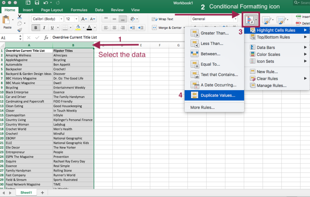
- From the conditional formatting menu, select “Highlight Cells Rules”. From the next menu that pops up, select “Duplicate Values…”. A grey box with a number of drop down options will appear. You can leave all of the drop down options as is. I opted to change the “Format With …” option to “yellow fill with dark yellow text”.
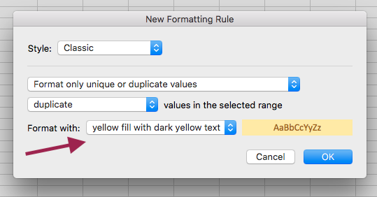
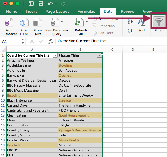
- Click the OK button. The duplicate data will now be highlighted in yellow fill as that was the formatting I selected. If nothing is highlighted, then the condition has not been met and no duplicate data is present.
- Based on this new formatting, I would now like to filter out the duplicate titles. With the columns still selected and greyed out, select Data from the Menu. Then click on Filter. Drop down arrows should now appear on your column headers.
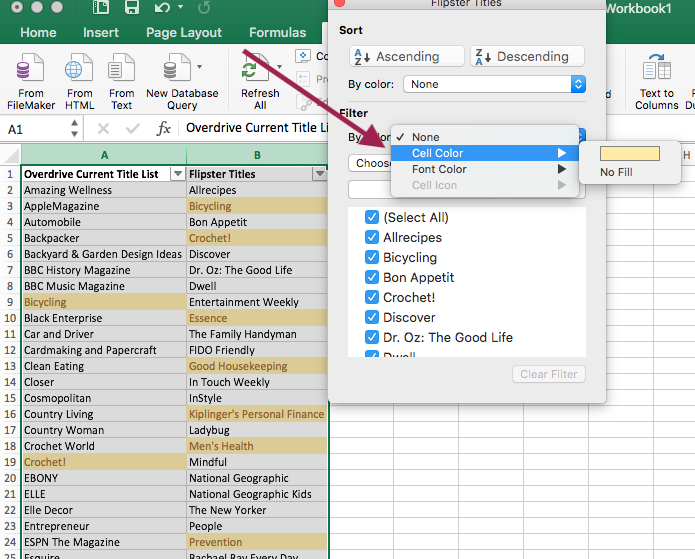
- On Column B, select the drop down arrow. In the pop up box, under Filter in the “By color:” field select the “Cell Color.” option. Then click the yellow box. In column B, only the cells highlighted in yellow should now be displaying. I have now identified the duplicate titles. These are the titles I need to remove from this supplier’s order.
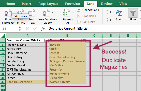
We can now remove the filter and conditional formatting rules from our worksheet.
- First let’s remove the filter. Click the Filter icon from the ribbon menu. The filter should now be removed.
- Click the “Home” tab to navigate back to the Home ribbon menu. Then click on the “Conditional Formatting” icon.
- Click “Clear Rules”. Then select “Clear Rules from Entire Sheet”.
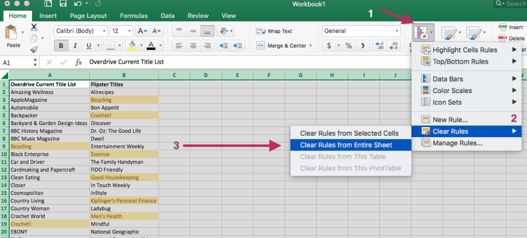
- All set! The worksheet should now be returned to its original formatting.
As noted earlier, conditional formatting can also be used to visualize trends. In the example below, a condition is set to highlight cells in green that have a value greater than 5,000.
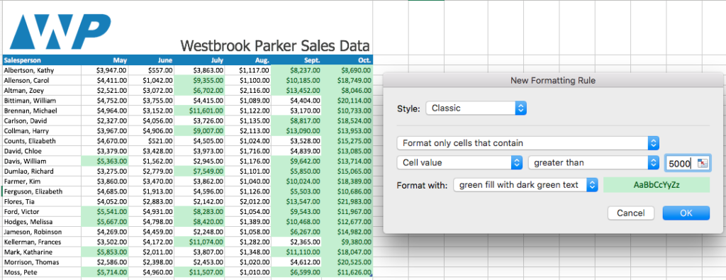
With the cells now being color coded, we can see the September and October were strong sales months.